A Dash of Maxwell’s

A Maxwell’s Equations Primer

Chapter IV – Equations Even a Computer Can Love

By Glen Dash, Ampyx LLC, GlenDash at alum.mit.edu

In the preceding chapters we have derived Maxwell’s Equations and expressed them in their “integral” and “differential” form. In different ways, both forms lend themselves to a certain intuitive understanding of the nature of electromagnetic fields and waves. In this installment, we will express Maxwell’s Equations in a their “computational form,” a form that allows our computers to do the work. To give you an idea where we are going, here are those equations:

Equation 1

Where:

E = Electric field in V/m

B = Magnetic flux density, B=mH

H = Magnetic field in Amps/m

V = Voltage

A = The “vector potential” (which we will explain shortly)

r_n = Charge density in Coulombs/m³ of a particular charge element, n

r_n = Distance from a given charge or current element, n, to the location of interest

v_n = Volume of a particular charge element, n

l_n = Length of a particular current element, n

a_n = Area of a particular current element, n

J_n = Total current density (both conductive and displacement) in amps/ m² of a particular current element, n

e, m = Permittivity and permeability respectively

We have added two elements we have not seen before: the gradient of the voltage (ÑV)and the “vector potential” (A). We will explain these terms in a moment, but for now note the following:

1. If we know the current density (J) at every point within a volume of interest, we can calculate the “vector potential” (A) by simple summation (Equation 1(d)). By taking the curl of the vector potential (A), we can derive the magnetic flux density (B), and hence the magnetic field (H) (Equation 1 (b)).

2. If we know the charge density (r) at every point within a volume of interest, we can calculate the voltage at every point (Equation 1(c)). We can calculate the electric field (E) by taking the gradient of the voltage and adding the time derivative of the vector potential (Equation 1(a)).

Obviously, to use these equations we will need to understand what we mean by the “gradient of the voltage” and the “vector potential” (A). To do that, there is a bit of additional math to master.

In Chapter III, we introduced two vector operations, the dot and cross product. The dot product of two vectors, R and S, computes the component of Vector R which is aligned with Vector S. The resultant is a scalar, not a vector. It is equal to:

By contrast, the cross product of two vectors is a vector itself. The cross product is equal to:

As indicated by the symbol ^, the direction of the cross product Vector T is determined by the right hand rule. The fingers of the right hand point from Vector R to Vector S, and the direction of the cross product T is indicated by the thumb of the right hand.

To these two operations, we now add a third, the gradient. As with the common usage of the term, the gradient is a slope. A steep hill has a large gradient, a small one a lesser gradient. The gradient of a function is itself a vector, that is at any point in within an area of interest it has both magnitude and direction. Mathematically, the gradient is equal to:

Where:

f = A scalar function of x, y and z

i, j, k = Unit vectors in the x, y and z directions respectively

Gradients are only applicable to scalar functions. These are functions which have a magnitude at every point within an area of interest, but no direction. A mountain can be described as a scalar function with the height at any point in within an area of interest being expressed as:

Where H_t equals the height of mountain in meters

If we want to know the slope of the mountain, we can mathematically compute it by taking the gradient.

It is conventional to write the gradient operation using the “del” operator. We introduced the del operator in our last installment. It is equal to:

We can multiply the del operator by our scalar height function to derive its gradient:

Known what is meant by the dot product, cross product, and gradient, we are now in a position to introduce “vector identities.” Vector identities are manipulations of the dot product, cross product, and gradient which can greatly speed up our mathematical analysis. For example, suppose we first take the cross product of two vectors R and S and then take the dot product of the resultant and Vector R. Mathematically, this would be expressed as:

A moment’s reflection, however, will reveal that the result of this operation is always equal to zero. The cross product of vectors R and S is a vector, T, whose direction is in a plane perpendicular to both R and S. Therefore, the dot product of R with T must equal zero. So we have the first of our vector identities shown in Table 1. For any two vectors R and S:

There are many more such vector identities that we could derive and which we will find useful. For example, both the dot product and the cross product are distributive. That is:

Further, multiplying a cross product of two vectors, R and S by -1 produces the same result as taking the cross product of R and -S:

Table 1 lists more vector identities. For the proofs of these, see Reference 1.

Table 1: Some Vector Identities.

As we described did in our previous chapter, we can always substitute the del operator for one of the vectors in our idenities. We will substitute the del operator for Vector R in Table 1 to produce Table 2, to which we will add a few more useful identities. Once again, for derivations of see Reference 1.

Table 2: Some vector identities using the “del” operator (Ñ) are shown. S and T are vector functions or fields, while f is a scalar function. Note that the gradient of a scalar is itself a vector function or field, so Ñf can be substituted for S or T in any of the above.

The first of the expressions making up the “computational” form of Maxwell’s Equations, Equation 1(a), is used to derive the electric field at any point within a volume of interest. The electric field is a function of voltage. Voltage is a scalar function, like the height of a mountain. At any point within a volume of interest it has magnitude, but no direction. We can take its gradient to produce vectors which give us the “slope” of the voltage. If the vector potential A in Equation 1(a) is unchanging, then:

This simply means that the electric field is equal to the gradient of the voltage when ¶A/¶t=0.

In one dimension:

Where:

DV = Voltage between two points, V₁ and V₂

Dx = Distance in meters between points 1 and 2

Or, equivalently for small Dx:

More generally in three dimensions:

What this says is that if we know the voltage at every point within a volume of interest and if A is unchanging, then we can derive the electric field.

To derive the voltage at any point within a volume of interest, it turns out that we only need to know where the electric charges are. This is illustrated in Figure 1. A number of charged spheres are shown suspended in space. Other than for these charged spheres, the space is empty. We will calculate the voltage at point P due to these charged spheres.

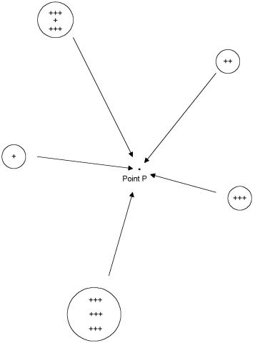
Figure 1: Where charges are static, the voltage at point P can be computed by summing the contributions of surrounding charges.

In the first chapter in this series, we calculated the work require to move a charge q from infinity to some point, such as point P in Figure 1. The work required is:

Where:

W= Work in joules

q = The charge being moved in Coulombs

Q_n = Charge on sphere n in Coulombs

r_n = Distance in meters from sphere n to point P in Figure 1

The work per unit charge moved (W/q) is equal to the voltage V, and is in units of Joules per Coulomb. The voltage at P is therefore:

We will find it convenient to re-express this equation in terms of charge density r rather than the total charge on a given sphere, Q_n. Charge density is simply the total charge on each sphere divided by its volume, v. So:

The vector potential A does not have the kind of readily measureable substance that an electric or magnetic field has. It is mostly just an mathematical tool. Mathematicians have defined the vector potential A as being a hypothetical field with the following characteristics:

In words rather than symbols, the curl of the vector potential is, by definition, equal to the magnetic flux density, and the divergence of A is everywhere equal to zero.

Before we move on to explore the usage of the vector potential, A, we will need to take yet another math detour. We will use some of our vector identities to manipulate Maxwell’s Equations.

We know that the differential form of the first of Maxwell’s equations is:

Since D=eE and, from Equation 1(a) E=-ÑV-¶A/¶t:

The last line is known as “Poisson’s Equation” and is usually written as:

Where:

In a region where there is no charge, r=0, so:

which is known as “Laplace’s Equation.” The operator Ñ² is known as the “Laplacian.”

From Maxwell’s fourth equation expressed in differential form, we can, with some difficulty, state the vector potential in terms of currents using our vector identities.

This derivation in may seem daunting, but we have see the form of the last line before. It is in the form of Poisson’s Equation. Therefore, we know that the solution is going to be – it is in the form of the solution to Poisson’s Equation. Poisson’s Equation states:

And we have already derived this expression for V.

So we can simply substitute the A for V and mJ for r/e and we have the solution for the vector potential, A, in terms of the total current density, J:

Where v_n = l_n a_n (volume equals length times area).

We can also break both the vector potential A and the current density J into their Cartesian components:

This equation tells us that the vector potential is aligned with the currents that produce it. If we sum the currents flowing in the x direction as shown in the equation, we will be able to calculate the vector potential in the x direction at any particular point of interest. The same is true for the vector potential in the y and z directions. That means that the vector potential A, like the scalar potential V, can be derived by mere addition, multiplication and division, things a computer does handily.

The last piece of the puzzle requires relating the vector potential A to the electric field E. To do this we will use that time-honored tradition in mathematics, propose a solution and plug it into our equations to see if it works. The solution that we will propose which relates A to E is:

We will test this solution by plugging it into the third of Maxwell’s Equations:

Having verified the relationship between the vector potential A and the electric field E, we can now state Maxwell’s Equations in their computational form, which, of course is where we started:

Before moving on, we should note one caveat. These equations assume that the effects of changing charges and currents are felt throughout the volume of interest instantaneously. That is, of course, not true, the effects propagate outward at a finite speed. In the next chapter we will adapt these equations to deal with finite propagation speeds using the theory of “retarded currents.” Then we will act as the computer and calculate by hand the near and far field radiation from a short length of wire. That short length of wire will, in turn, become our building block for the powerful Method of Moments which we will introduce in the chapters to come.

References

1. Spiegel, M., Vector Analysis and an Introduction to Tensor Analysis, Schaum’s Outline Series, McGraw Hill, 1959.

2. Kraus, J., Electromagnetics, Fourth Edition, McGraw Hill, 1992.